Overview
- Newtonian Fluids
- Basic Equations
- Riemann Solvers
- Special Relativistic Fluids
- Basic Equations
- Riemann Solvers
- Numerics
Basic Equations (Newtonian)
Euler's equations (EEs)
where
EEs in conservative form
which can be written as
\[ \partial_t \vec{U} + \nabla \cdot [\vec{F}(\vec{U})] = \vec{S} \]Examples of source terms, $\vec{S}$
- External forces such as gravity
- Radiative heating / cooling: happen on shorter timescales than the fluid dynamics modeled
- Ionization, chemical kinetics: ion species not individually conserved
- Geometric source terms: appear when transforming into curvlinear coordinates
Finite Volume Methods (1D)
The conservative EEs in integral form are
\[ \frac{d}{dt} \int_{x_1}^{x_2} U(x, t)dx = F[U(x_1,t)] - F[U(x_2,t)] \]which, over one grid cell in a single time step, gives
\[ \begin{aligned} & \int_{x_{i-1/2}}^{x_{i+1/2}}U(x, t_{n+1})dx - \int_{x_{i-1/2}}^{x_{i+1/2}}U(x, t_n)dx\\ & ~~~= \int_{t_n}^{t_{n+1}}F[U(x_{i-1/2},t)]dt - \int_{t_n}^{t_{n+1}}F[U(x_{i+1/2},t)]dt; \end{aligned} \]If we define some average conserved quantity, $\bar{U}$, such that
$$ \bar{U}_i^{n} \approx \frac{1}{\Delta x} \int_{\mathcal{X}_i} U(x, t_n)dx; ~ \mathcal{X}_i = [x_{i-1/2}, x_{i+1/2}] $$then we can rewrite the integral form from before as
$$ \bar{U}_i^{n+1} = \bar{U}_i^n - \frac{\Delta t}{\Delta x}(\bar{F}^n_{i+1/2} - \bar{F}^n_{i-1/2}) $$where
$$ \bar{F}_i^n \approx \frac{1}{\Delta t} \int_{t_n}^{t_{n+1}}F[U(x_i,t)]dt $$Pictorially, series of Riemann problems
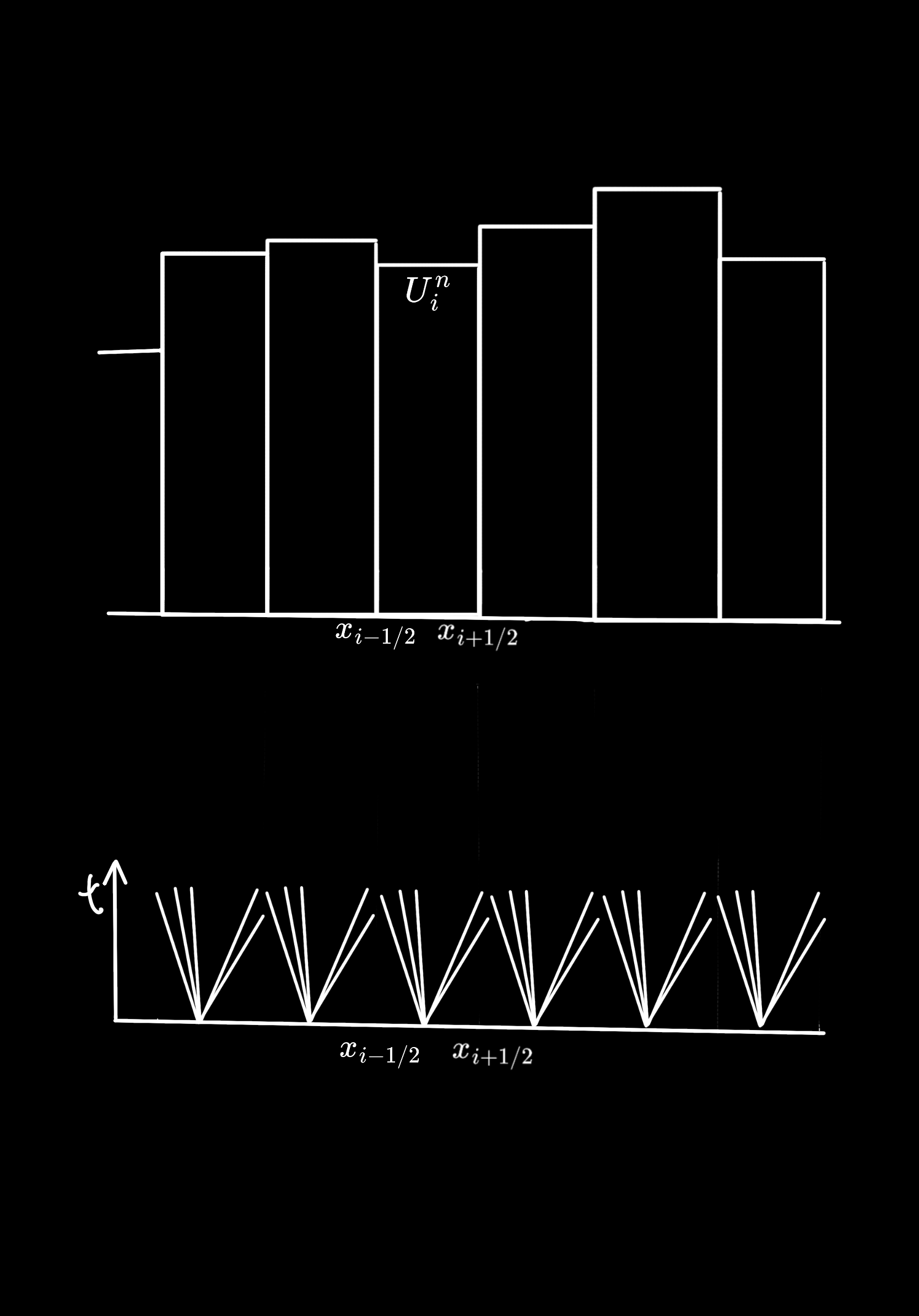
Similarity solution
If $U^*(U_L,U_R)$ is the exact solution to the Riemann problem along the ray $x/t$ given the data:
$$ U(x, 0) = \begin{cases} U_L & \text{if}~~ x < 0\\ U_R & \text{if}~~ x> 0 \end{cases} $$then
$$ \tilde{U}^n(x_i,t) \equiv U^*(U^n_{i-1}, U^n_i) $$for all $t \in [t_n, t_{n+1}$] as long as $\Delta t$ is small enough (?).
Stability: Linear wave problem
Let $F = aU$, then
$$ U_i^{n+1} = U_i^{n} - a \frac{\Delta t}{\Delta x}(U^n_i - U^{n}_{i-1}) $$which requires $|a \frac{\Delta t}{\Delta x}| \leq 1$. This is the Courant-Friedrichs-Lewy (CFL) stability condition. More generally, the stability condition is
$$ \left| a \frac{\Delta t}{\Delta x} \right| \leq C_{\rm max}; ~~ C_{\rm max} = 1~~\text{if using explicit solver} $$Pictorially, HLL
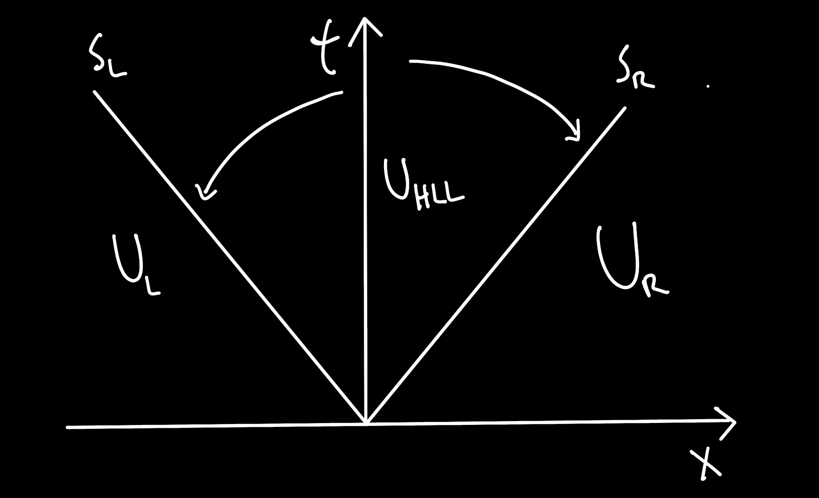
The HLL state
given some signal velocities, $s_L$ and $s_R$, integrating \[ \begin{aligned} & \int_{x_{i-1/2}}^{x_{i+1/2}}U(x, t_{n+1})dx - \int_{x_{i-1/2}}^{x_{i+1/2}}U(x, t_n)dx\\ & ~~~= \int_{t_n}^{t_{n+1}}F[U(x_{i-1/2},t)]dt - \int_{t_n}^{t_{n+1}}F[U(x_{i+1/2},t)]dt \end{aligned} \] gives the intermediate state $$ U_{\rm HLL} = \frac{s_R U_R - s_L U_L + F_L - F_R}{s_R - s_L} $$
HLLC, pictorially
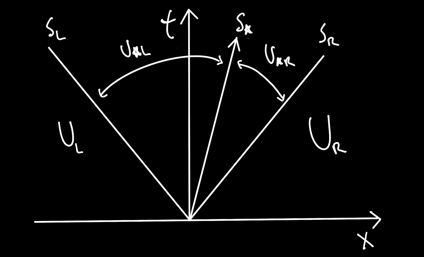
Noticing the difference
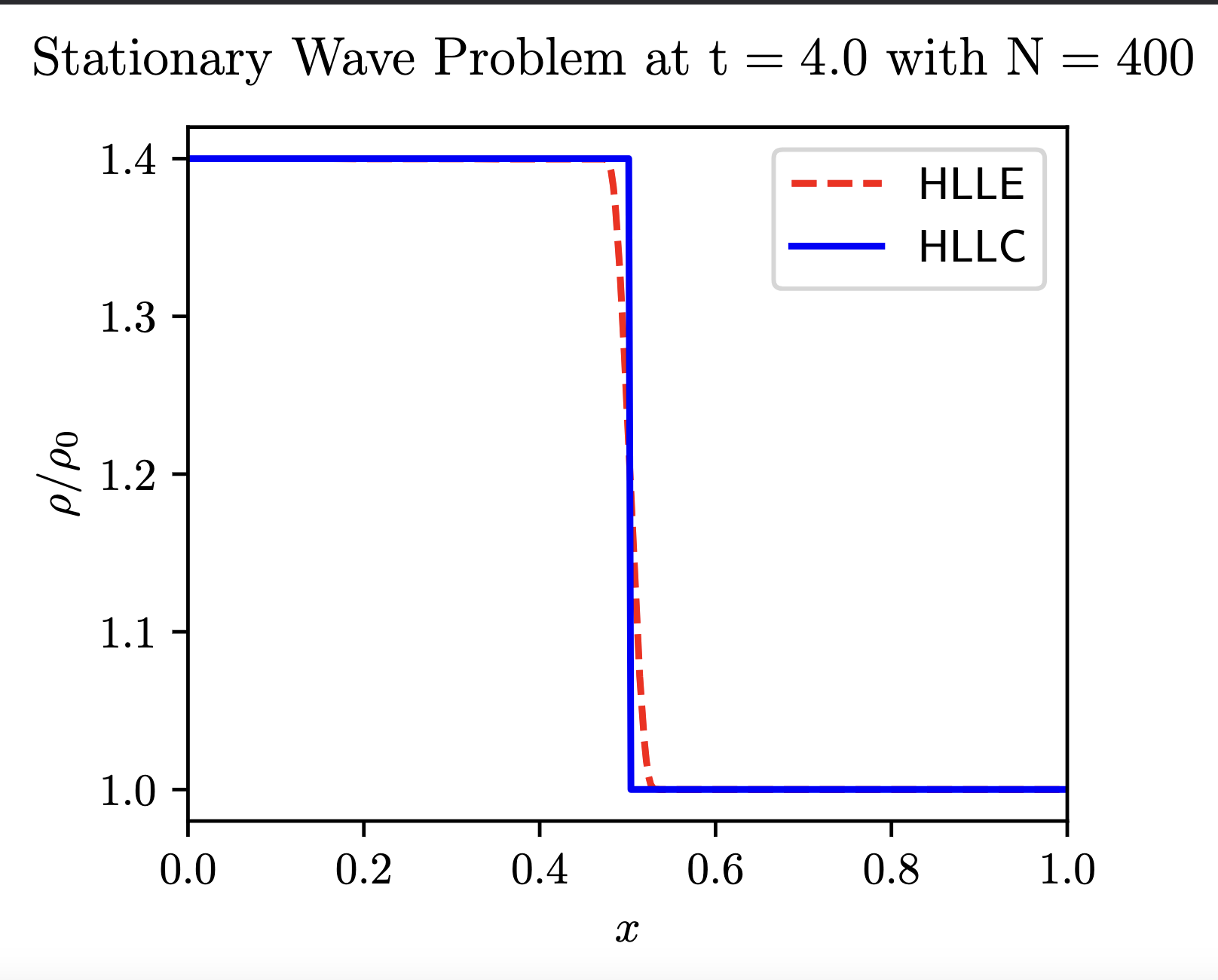
Implementation
Usually we define a vector of primitive variables, $W$, that all of the conservative variables, $U$, are derived from. Namely, $$ W = \begin{pmatrix} \rho \\ \vec{v} \\ p \end{pmatrix}~~ \text{so that}~~ U = \begin{pmatrix} W_\rho\\ W_\rho W_{v}\\ W_p / (\gamma - 1) + W_\rho W_v^2 \end{pmatrix} $$
Implementation: Some Definitions (C++)
						constexpr double gamma_ad = 5.0 / 3.0;
						struct Primitive {
							double rho, v1, v2, v3, pre;
							/**
							Helper Functions
							...
							**/
						};
						struct Conserved {
							double rho, m1, m2, m3, nrg;
							/**
							Helper Functions
							...
							**/
						};
						struct Eigenvals {
							double sL, sR;
						}
Implementation: Cons2Prim & Prim2Cons (C++)
						Conservative prims2cons (const Primitive &w) {
							double vsq = w.v1 * w.v1 + w.v2 * w.v2 + w.v3 + w.v3;
							return {
								w.rho,
								w.rho * w.v1,
								w.rho * w.v2,
								w.rho * w.v3,
								w.pre / (gamma_ad - 1.0) + 0.5 * w.rho * vsq
							};
						};

						Primitive cons2prim (const Conservative &u) {
							double v1 = u.m1 / u.rho;
							double v2 = u.m2 / u.rho;
							double v3 = u.m3 / u.rho;
							double vsq = v1 * v1 + v2 * v2 + v3 * v3;
							double pre  = (gamma_ad - 1.0) * (w.nrg - 0.5 * w.rho * vsq);
							return {
								w.rho,
								v1,
								v2,
								v3,
								pre
							};
						};
Implementation: Fluxes (C++)
					Conservative calc_hll_flux (/* variables */) {
							// this just returns (vL - cs, vR + cs)
							const auto lambda = calc_eigenvals(left_prims, right_prims);

							const double sL   = lambda.sL;
							const double sR   = lambda.sR;

							// Compute the HLL Flux component-wise
							if (0.0 <= sL) {
								return left_flux;
							}
							else if (0.0 >= sR) {
								return right_flux;
							}
							else {
								return (left_flux * sR - right_flux * sL +
													(right_state - left_state) * sR * sL) /
												(sR - sL);
							}
						};

					Conservative calc_hllc_flux (/* variables */) {
							// this now returns (vL - cs, vR + cs, aStar, pStar)
							const auto lambda = calc_eigenvals(left_prims, right_prims);

   				const double sL     = lambda.sL;
							const double sR     = lambda.sR;

							// Quick checks before moving on with rest of computation
							if (0.0 <= sL) {
								return left_flux;
							}
							else if (0.0 >= sR) {
								return right_flux;
							}

							const double aStar = lambda.aStar;
							const double pStar = lambda.pStar;

							const auto hll_flux = (left_flux * sR + right_flux * sL -
											(right_state - left_state) * sL * sR) /
											(sL + sR);

							const auto hll_state =
								(right_state * sR - left_state * sL - right_flux + left_flux) /
								(sR - sL);

							if (0.0 <= aStar) {
								double pressure = left_prims.pre;
								double v        = left_prims.v1;
								double rho      = left_state.rho;
								double m        = left_state.m1;
								double energy   = left_state.nrg;
								double cofac    = 1.0 / (sL - aStar);

								double rhoStar = cofac * (sL - v) * rho;
								double mstar   = cofac * (m * (sL - v) - pressure + pStar);
								double eStar =
									cofac * (energy * (sL - v) + pStar * aStar - pressure * v);

								auto star_state = Conserved{rhoStar, mstar, eStar};

								// Compute the intermediate left flux
								return left_flux + (star_state - left_state) * sL -
									star_state * vface;
							}
							else {
								double pressure = right_prims.pre;
								double v        = right_prims.v1;
								double rho      = right_state.rho;
								double m        = right_state.m1;
								double energy   = right_state.nrg;
								double cofac    = 1.0 / (sR - aStar);

								double rhoStar = cofac * (sR - v) * rho;
								double mstar   = cofac * (m * (sR - v) - pressure + pStar);
								double eStar =
									cofac * (energy * (sR - v) + pStar * aStar - pressure * v);

								auto star_state = Conserved{rhoStar, mstar, eStar};

								// Compute the intermediate right flux
								return right_flux + (star_state - right_state) * sR -
									star_state * vface;
							}
Implementation: Update (C++)
							const Conserved f_rf = calc_hllc_flux(/* depends on i, and i+1 cells */);
							const Conserved f_lf = calc_hllc_flux(/* depends on i, and i-1 cells */);

							// update the conserved vector at cell i
							u[i] -= dt * (f_rf - f_lf) / dx;
Regime of Applicability
- Non-relativistic blast waves
- Accretion problems
- Hydrodynamic bow shock problems
- Most strong shock problems
Basic Equations (Relativistic)
Special Relativistic Hydrodynamics (SRHD)
where
SRHD in conservative form
with $\tau = \rho h \Gamma^2 - p - \Gamma \rho$. The above can still be written as
\[ \partial_t \vec{U} + \nabla \cdot [\vec{F}(\vec{U})] = 0 \]Difference from Newtonian
Almost everything is the same as before except now you have $$ \Gamma = (1 - v^2)^{-1/2} $$ which couples the velocity terms to all equations, so we now have a non-linear (in $\Gamma$) equation for the pressure: $$ \tau + \Gamma \rho + p = \rho \Gamma^2 + \frac{\gamma}{\gamma - 1}p \Gamma^2 $$ which can be solved using a root finding algorithm.
Implementation
Usually we define a vector of primitive variables, $W$, that all of the conservative variables, $U$, are derived from. Namely, $$ W = \begin{pmatrix} \rho \\ \vec{v} \\ p \end{pmatrix}~~ \text{and}~~ U = \begin{pmatrix} \rho \Gamma := D \\ \rho h \Gamma^2 \vec{v} := \vec{M}\\ \tau \end{pmatrix} $$
Implementation: Some Definitions (C++)
						constexpr double gamma_ad = 4.0 / 3.0;
						struct Primitive {
							double rho, v1, v2, v3, pre;
							/**
							Helper Functions
							...
							**/
						};
						struct Conserved {
							double rho, m1, m2, m3, nrg;
							/**
							Helper Functions
							...
							**/
						};
						struct Eigenvals {
							double sL, sR;
						}
Implementation: Cons2Prim & Prim2Cons (C++)
						Conservative prims2cons (const Primitive &w) {
							double vsq = w.v1 * w.v1 + w.v2 * w.v2 + w.v3 + w.v3;
							double lorentz = 1 / std::sqrt(1.0 - vsq);
							double h = 1.0 + w.p * gamma_ad / (w.rho * (gamma_ad - 1.0));
							double tau = w.rho * h * lorentz * lorentz - w.p - lorentz * w.rho;
							return {
								w.rho * lorentz,
								w.rho * h * lorentz * lorentz * w.v1,
								w.rho * h * lorentz * lorentz * w.v2,
								w.rho * h * lorentz * lorentz * w.v3,
								tau
							};
						};

						Primitive cons2prim (const Conservative &u) {
							/* Details */
							do {
								// compute x_[k+1]
								f = newton_f(gamma, tau, d, m, peq);
								g = newton_g(gamma, tau, d, m, peq);

								// newton_f = (gamma_ad - 1.0) * rho * eps - p;
								// newton_g = cs^2 * v^2 - 1.0 (Aloy et al. 1999)
								peq -= f / g;

								if (iter >= global::MAX_ITER || std::isnan(peq)) {
									troubled_data[gid] = 1;
									dt                 = INFINITY;
									inFailureState     = true;
									found_failure      = true;
									break;
								}
								iter++;

							} while (std::abs(f / g) >= tol);

							const double inv_et = 1.0 / (tau + d + peq);
							const double v1     = m1 * inv_et;
							const double lorentz= 1.0 / std::sqrt(1.0 - v1 * v1);
							return {d / lorentz, v1, peq};
						};
Implementation: Fluxes (C++)
					Conservative calc_hll_flux (/* variables */) {
							// this returns wavespeeds according
							// to Eq. 23 in Mignone and Bodo (2005)
							const auto lambda = calc_eigenvals(left_prims, right_prims);

							const double sL   = lambda.sL;
							const double sR   = lambda.sR;

							// Compute the HLL Flux component-wise
							if (0.0 <= sL) {
								return left_flux;
							}
							else if (0.0 >= sR) {
								return right_flux;
							}
							else {
								return (left_flux * sR - right_flux * sL +
													(right_state - left_state) * sR * sL) /
												(sR - sL);
							}
						};

					Conservative calc_hllc_flux (/* variables */) {
							// this now returns (vL - cs, vR + cs, aStar, pStar)
							const auto lambda = calc_eigenvals(left_prims, right_prims);

   				const double sL     = lambda.sL;
							const double sR     = lambda.sR;

							// Quick checks before moving on with rest of computation
							if (0.0 <= sL) {
								return left_flux;
							}
							else if (0.0 >= sR) {
								return right_flux;
							}

							const double aStar = lambda.aStar;
							const double pStar = lambda.pStar;

							const auto hll_flux = (left_flux * sR + right_flux * sL -
											(right_state - left_state) * sL * sR) /
											(sL + sR);

							const auto hll_state =
								(right_state * sR - left_state * sL - right_flux + left_flux) /
								(sR - sL);

							if (0.0 <= aStar) {
								double pressure = left_prims.pre;
								double v        = left_prims.v1;
								double rho      = left_state.rho;
								double m        = left_state.m1;
								double energy   = left_state.nrg;
								double cofac    = 1.0 / (sL - aStar);

								double rhoStar = cofac * (sL - v) * rho;
								double mstar   = cofac * (m * (sL - v) - pressure + pStar);
								double eStar =
									cofac * (energy * (sL - v) + pStar * aStar - pressure * v);

								auto star_state = Conserved{rhoStar, mstar, eStar};

								// Compute the intermediate left flux
								return left_flux + (star_state - left_state) * sL -
									star_state * vface;
							}
							else {
								double pressure = right_prims.pre;
								double v        = right_prims.v1;
								double rho      = right_state.rho;
								double m        = right_state.m1;
								double energy   = right_state.nrg;
								double cofac    = 1.0 / (sR - aStar);

								double rhoStar = cofac * (sR - v) * rho;
								double mstar   = cofac * (m * (sR - v) - pressure + pStar);
								double eStar =
									cofac * (energy * (sR - v) + pStar * aStar - pressure * v);

								auto star_state = Conserved{rhoStar, mstar, eStar};

								// Compute the intermediate right flux
								return right_flux + (star_state - right_state) * sR -
									star_state * vface;
							}
Implementation: Update (C++)
							const Conserved f_rf = calc_hllc_flux(/* depends on i, and i+1 cells */);
							const Conserved f_lf = calc_hllc_flux(/* depends on i, and i-1 cells */);

							// update the conserved vector at cell i
							u[i] -= dt * (f_rf - f_lf) / dx;
Regime of Applicability
- Relativistic blast waves
- Astrophysical jets
- Relativistic turbulence
- Extreme temperaures / shock jump problems
Something to note --- Relativistic problems with large $\Gamma$ must be very high resolution since:
- a spherical blast wave is Lorentz contracted by $R / \Gamma^2$
- Usually, a very small amount of mass is accelerated to high $\Gamma$
otherwise, your simulation can just crash or give a wrong result.
Setups
Setting up a problem
Setting up a problem is code-specific, so I will only show how to do it with simbi
What is simbi?
3D Relativistic MHD, GPU-Accelerated moving mesh gas dynamics code with the following features:
- Eulerian in Cartesian, Cylindrical, and Spherical
- CPU / GPU agnostic
- User-defined mesh motion as well as dynamic BCs
- Same code runs on Nvidia and AMD GPUs
- C++ backend with a Python front end
- Immersed boundary on top of grid (Peskin 2002)
- Passive scalars
- Can make synchrotron light curves and sky maps in post processing
How do I set up a problem in simbi?
Ex: Sod Problem
from simbi import BaseConfig, DynamicArg, simbi_property
from simbi.key_types import *

class SodProblem(BaseConfig):
    """
    Sod's Shock Tube Problem in 1D Newtonian Fluid
    """
    nzones    = DynamicArg("nzones", 1000, help="number of grid zones", var_type=int)
    ad_gamma  = DynamicArg("ad-gamma", 5.0 / 3.0, help="Adiabatic gas index", var_type = float)

    @simbi_property
    def initial_state(self) -> Sequence[Sequence[float]]:
        return ((1.0, 0.0, 1.0), (0.125, 0.0, 0.1))

    @simbi_property
    def geometry(self) -> Sequence[float]:
        return (0.0, 1.0, 0.5)

    @simbi_property
    def x1_cell_spacing(self) -> str:
        return "linear"

    @simbi_property
    def coord_system(self) -> str:
        return "cartesian"

    @simbi_property
    def resolution(self) -> DynamicArg:
        return self.nzones

    @simbi_property
    def gamma(self) -> DynamicArg:
        return self.ad_gamma

    @simbi_property
    def regime(self) -> str:
        return "classical"
Running it
where options can be
for example. There's many more.
Output of "simbi run sod ..."
(base) ~/research/simbi/ [develop*] simbi run sod --omp -p 1
--------------------------------------------------------------------------------
Validating Config Script Type Safety...
Success: no issues found in 1 source file
--------------------------------------------------------------------------------
Initializing Problem With a 1D Discontinuity...

Problem Parameters:
================================================================================
ad-gamma...................... 1.667           Adiabatic gas index
nzones........................ 1000            number of grid zones
================================================================================

    Sod's Shock Tube Problem in 1D Newtonian Fluid

================================================================================
================================================================================
Simulation Parameters
================================================================================
tstart........................ 0.000
tend.......................... 1.000
dlogt......................... 0.000
plm_theta..................... 1.500
x1_cell_spacing............... linear
x2_cell_spacing............... linear
x3_cell_spacing............... linear
cfl........................... 0.100
sources....................... None
gsources...................... None
bsources...................... None
passive_scalars............... None
solver........................ hllc
chkpt......................... None
chkpt_interval................ 0.100
data_directory................ data/
boundary_conditions........... outflow
engine_duration............... 0.000
compute_mode.................. omp
quirk_smoothing............... False
constant_sources.............. False
scale_factor.................. None
scale_factor_derivative....... None
dens_outer.................... None
mom_outer..................... None
edens_outer................... None
object_positions.............. None
boundary_sources.............. None
spatial_order................. plm
time_order.................... rk2
adiabatic_gamma............... 1.67
resolution.................... (1000,)
geometry...................... (0.0, 1.0, 0.5)
coord_system.................. cartesian
regime........................ srhd
================================================================================
2024-03-14 14:02:05,328 - SIMBI - DEBUG - Using OpenMP multithreading

Loading... ━━━━━━━━━━━━━━━━━━━━━━━━━━━━━━━━━━━━━━━━ 100% 0:00:01
================================================================================
Computing solution using PLM in space, RK2 in time...
================================================================================
CPU Compute Thread(s): 8

[Writing File...: data/1000.chkpt.000_000.h5]
iteration:  1300    dt: 7.25e-05    time: 9.43e-02    zones/sec: 4.60e+06 [==>                         ] 9 %
[Writing File...: data/1000.chkpt.000_100.h5]
iteration:  2700    dt: 7.25e-05    time: 1.96e-01    zones/sec: 4.29e+06 [=====>                      ] 19 %
[Writing File...: data/1000.chkpt.000_200.h5]
iteration:  4100    dt: 7.25e-05    time: 2.97e-01    zones/sec: 5.19e+06 [========>                   ] 29 %
[Writing File...: data/1000.chkpt.000_300.h5]
iteration:  5500    dt: 7.25e-05    time: 3.99e-01    zones/sec: 4.04e+06 [===========>                ] 39 %
[Writing File...: data/1000.chkpt.000_400.h5]
iteration:  6800    dt: 7.25e-05    time: 4.93e-01    zones/sec: 3.74e+06 [=============>              ] 49 %
[Writing File...: data/1000.chkpt.000_500.h5]
iteration:  8200    dt: 7.25e-05    time: 5.95e-01    zones/sec: 4.27e+06 [================>           ] 59 %
[Writing File...: data/1000.chkpt.000_600.h5]
iteration:  9900    dt: 5.70e-05    time: 6.95e-01    zones/sec: 3.93e+06 [===================>        ] 69 %
[Writing File...: data/1000.chkpt.000_700.h5]
iteration: 11700    dt: 5.70e-05    time: 7.98e-01    zones/sec: 4.35e+06 [======================>     ] 79 %
[Writing File...: data/1000.chkpt.000_800.h5]
iteration: 13400    dt: 5.70e-05    time: 8.94e-01    zones/sec: 4.46e+06 [=========================>  ] 89 %
[Writing File...: data/1000.chkpt.000_900.h5]
iteration: 15200    dt: 5.70e-05    time: 9.97e-01    zones/sec: 3.58e+06 [===========================>] 99 %
[Writing File...: data/1000.chkpt.001_000.h5]

Average zone update/sec for 15253 iterations was 4.32e+06 zones/sec
Visualizing
simbi plot data/1000.chkpt* --field rho p v
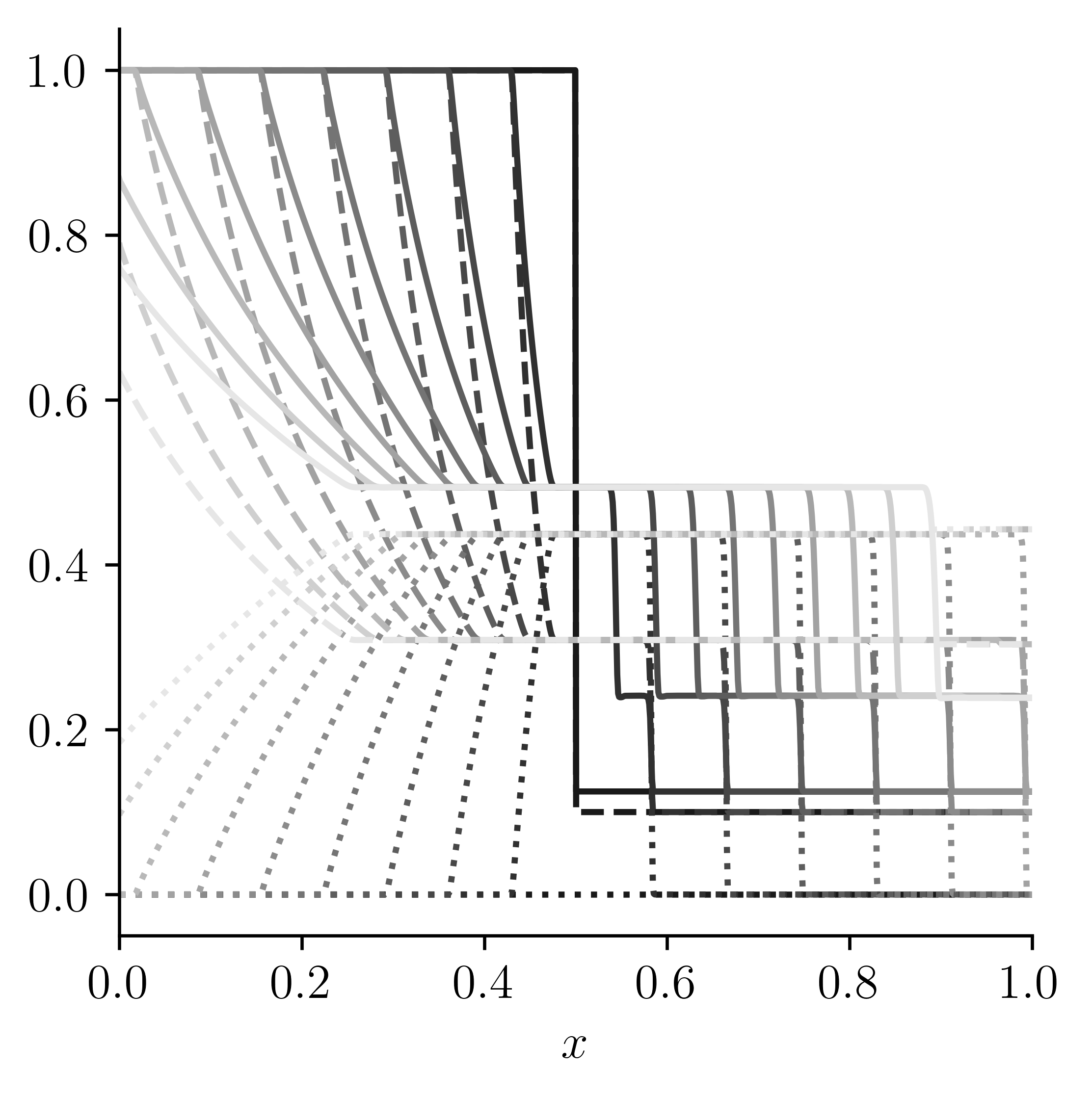
Visualizing, moving mesh
simbi plot data/marti_muller/1000.chkpt* --field d p u --kind movie
Visualizing, 2D shock tube
simbi plot data/quad_shocktube/400.chkpt* --field d --kind movie --log
Visualizing, astrophysical jet
simbi plot data/jet/2048.chkpt* --field d --kind movie --pictorial --dbg
Places simbi was used for science
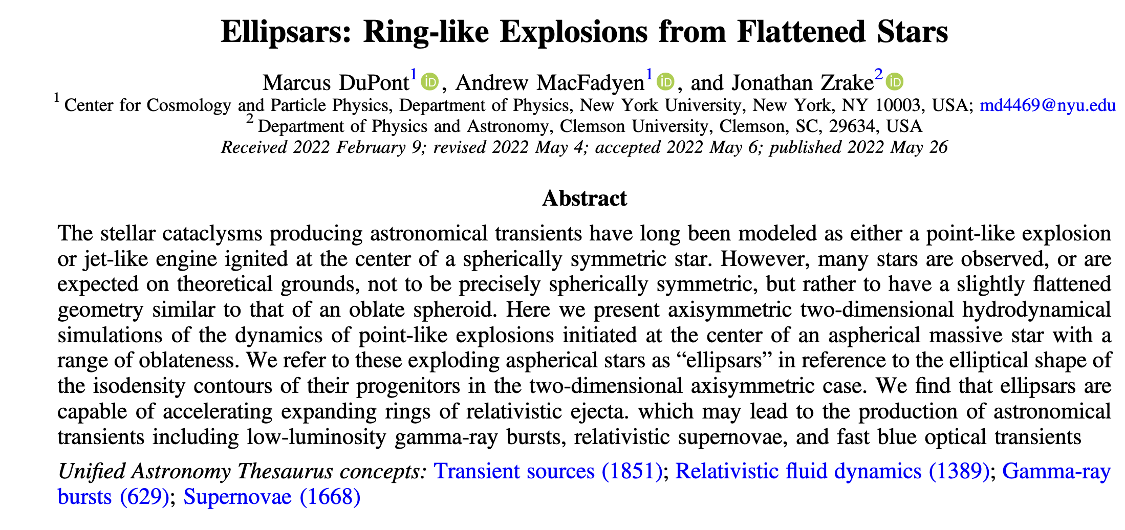
Places simbi was used for science
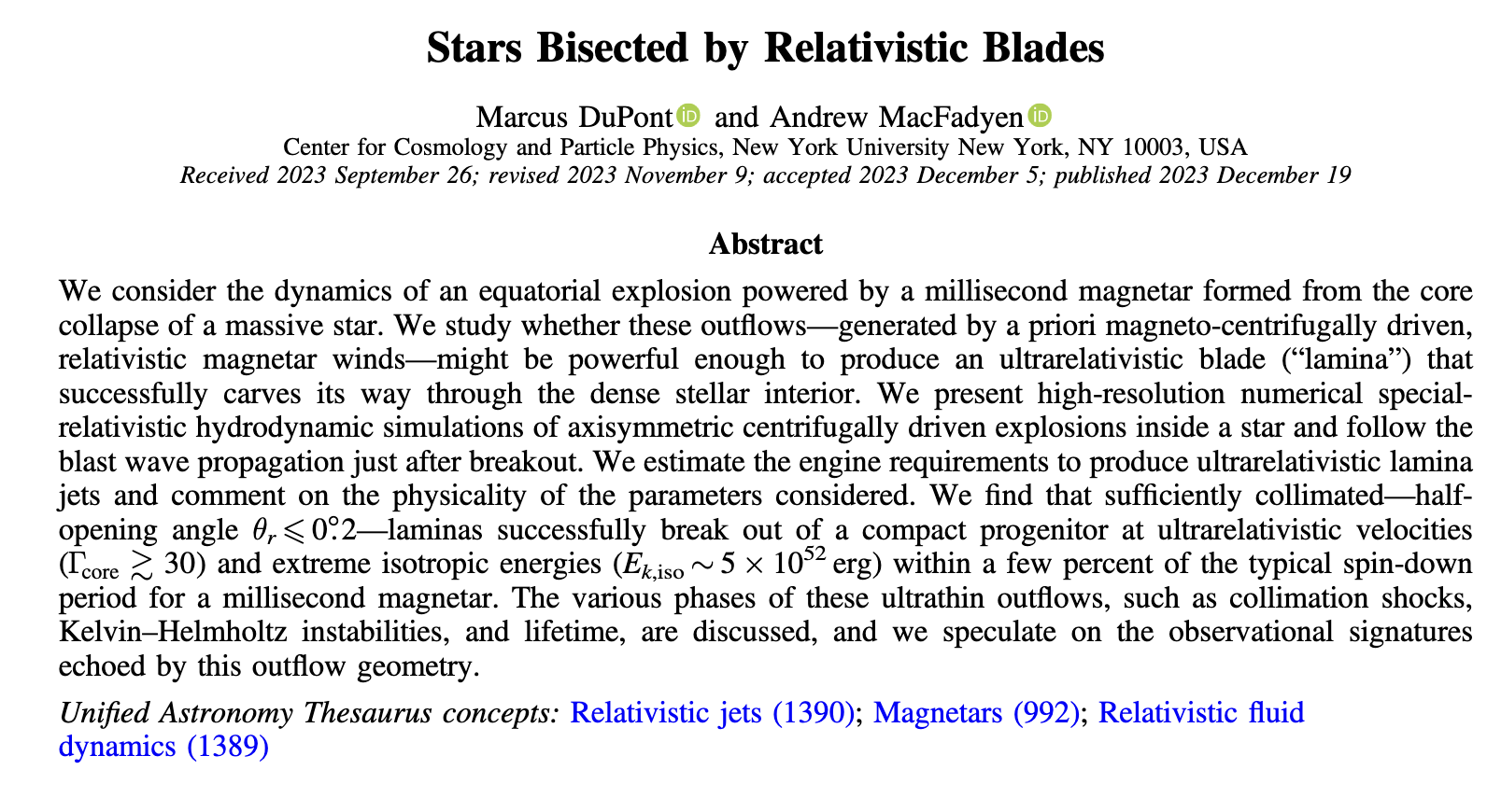
Places simbi was used for science

Places simbi was used for science
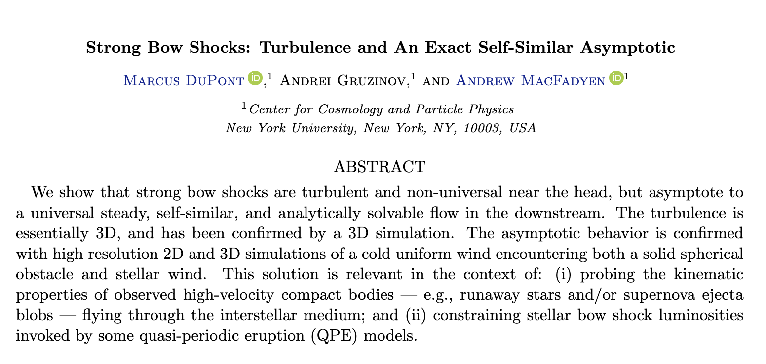
Dicussion Time (Thank You!)
Just in case
- GPUs *can* be an order of magnitude faster than CPU problems
- GPUs on a single node can know about each other's memory
- GPUs now support hash maps (lookup tables), so detailed EoS should be possible
Code base
git repo